import numpy as np
from iminuit import Minuit
from iminuit.cost import ExtendedUnbinnedNLL
from numba_stats import uniform_pdf, norm_pdf
import matplotlib.pyplot as plt
import boost_histogram as bhThis is an attempt to clear up the confusion around p-value computation and based on the authorative source on that matter:
G. Cowan, K. Cranmer, E. Gross, O. Vitells, Eur.Phys.J.C 71 (2011) 1554
The point of that paper is that one should use two different test statistics based on the likelihood-ratio for deviations that are always positive and for deviations where the sign is not known a priori. One gets two different p-values accordingly. The conversion to significance is then always the same.
I generate a flat distribution from \((-1,1)\) which represents background-only samples, then I fit a Gaussian peak centered at 0 with width 0.1 to this data test the two hypotheses
- \(H_0\): there is only background
- \(H_1\): there is background and a signal
The \(H_1\) in these kinds of tests is never arbitrary in terms of the signal, we do not seek for any deviation, but a rather specific one. In our example, we seek for a signal in particular location (here centered at 0). This is important for the computation of the p-value later. The less constrained \(H_1\) is, the more of the Look-Elsewhere Effect I get, because more random fluctuations of the background can be confused with a signal.
When fitting the toys, I allow the amplitude \(\mu\) of the signal to be positive or negative (following Cowan et al.). As a test statistic for a deviation from the background-only case I use \(t_0\) (again following Cowan et al. in the notation) \[ t_0 = -2\ln \lambda(0) = -2 \ln \frac{L(0, \hat {\hat \theta})}{L(\hat \mu, \hat \theta)} \] where * \(\mu\) is the amplitude of the hypothetical signal * \(\theta\) are nuisance parameters * \(\hat \mu\) is the fitted value of \(\mu\) * \(\hat\theta\) are the fitted values of \(\theta\) when \(\mu\) is also fitted * \(\hat{\hat\theta}\) are the fitted values of \(\theta\) under the condition \(\mu = 0\).
If you search for \(t_0\) in the paper, it is not explicitly written there, \(t_0\) is \(t_\mu\) from section 2.1 with \(\mu = 0\).
rng = np.random.default_rng(1)

def model(x, mu, theta):
    return mu + theta, mu * norm_pdf(x, 0, 0.1) + theta * uniform_pdf(x, -1, 2)

positive = [0]
negative = [0]
t0 = []
mu = []
for imc in range(1000):
    b = rng.uniform(-1, 1, size=1000)
    c = ExtendedUnbinnedNLL(b, model)
    m = Minuit(c, mu=0, theta=len(b))
    m.limits["theta"] = (0, None)
    m.fixed["mu"] = True
    m.migrad()
    assert m.valid
    lnL_b = -m.fval
    m.fixed["mu"] = False
    m.migrad()
    mui = m.values["mu"]
    lnL_sb = -m.fval
    t0i = 2 * (lnL_sb - lnL_b)
    t0.append(t0i)
    mu.append(mui)
    if mui > 0 and t0i > positive[0]:
        h = bh.Histogram(bh.axis.Regular(100, -1, 1))
        h.fill(b)
        positive = (t0i, h, m.values[:], m.covariance[:])
    elif mui < 0 and t0i > negative[0]:
        h = bh.Histogram(bh.axis.Regular(100, -1, 1))
        h.fill(b)
        negative = (t0i, h, m.values[:], m.covariance[:])

t0 = np.array(t0)
mu = np.array(mu)
Let’s look at the two most extreme deviations from \(H_0\), the ones with the largest and smallest signal.
fig, ax = plt.subplots(1, 2, figsize=(14, 5), sharex=True, sharey=True)
for (t0i, h, par, cov), axi in zip((negative, positive), ax):
    plt.sca(axi)
    scale = 1/h.axes[0].widths
    plt.errorbar(h.axes[0].centers, h.values() * scale, h.variances()**0.5 * scale, fmt="ok", label="data")
    scale = 1 / h.axes[0].widths
    xm = np.linspace(-1, 1)
    plt.plot(xm, model(xm, *par)[1], label="fit")
    plt.legend()
    dev = par[0] / cov[0,0] ** 0.5
    plt.title(f"$\mu = {par[0]:.1f}$        $t_0 = {t0i:.2f}$")
    plt.ylabel("density")
    plt.xlabel("$x$")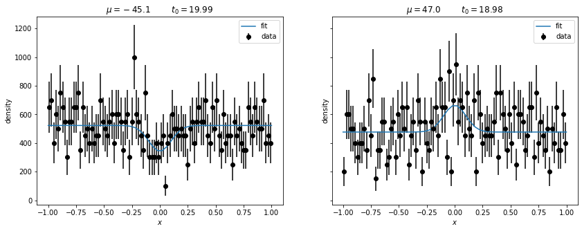
Both upward and downward fluctuations are unlikely events if \(H_0\) is true and therefore both get a large value of our test statistic \(t_0\), which does not know in which way the deviation went.
Searches with \(\mu > 0\) (for a new particle, new decay mode, etc.)
In most cases we look for a positive peak (new particle, new decay mode, etc). If we see a downward fluctuation, we know for sure that this cannot be what we are looking for. Therefore, when we compute the p-value for some observation from a simulation like this one, we must not regard large values of the test statistic when the fluctuation was negative, since this is not a deviation of \(H_0\) that mimics our signal. Instead we should set \(t_0\) to zero in such cases. Cowan et al. use \(q_0\) for this modified test statistic \[ q_0 = \begin{cases} t_0 &\text{if } \hat\mu \ge 0 \\ 0 &\text{otherwise} \end{cases} \]
plt.hist(t0, alpha=0.5, bins=20, range=(0, 20), label="$t_0$")
q0 = t0.copy()
q0 = np.where(mu < 0, 0, t0)
plt.hist(q0, alpha=0.5, bins=20, range=(0, 20), label="$q_0$")
plt.legend()
plt.axhline()
plt.xlabel("$t_0, q_0$")
plt.semilogy();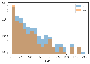
If we observed \(t_0 = q_0 = 15\) in a real experiment, we need to compare it with the \(q_0\) distribution and not with the \(t_0\) distribution to compute the p-value.
print(f"Wrong: p-value based on t0-distribution {np.mean(t0 > 15)}")
print(f"Right: p-value based on q0-distribution {np.mean(q0 > 15)}")
Wrong: p-value based on t0-distribution 0.006
Right: p-value based on q0-distribution 0.004As we can see, the p-value is enhanced in this case, because we do not need to consider the negative fluctuations at all. The conversion to significance \(Z\) is done with a normal distribution.
from scipy.stats import norm

p = np.mean(q0 > 15)
print(f"Z = {norm.ppf(1 - p):.2f}")
Z = 2.65Searches for deviations where the sign of \(\mu\) is not known a priori
If cannot exclude a priori that our signal has \(\mu < 0\), we need to use the \(t_0\) distribution instead of \(q_0\).
If we observed \(t_0 = 15\) in a real experiment, we need to compare it with \(t_0\) distribution to compute the p-value.
print(f"Right: p-value based on t0-distribution {np.mean(t0 > 15)}")Right: p-value based on t0-distribution 0.006As we can see, the p-value is diluted in this case, because we need to consider fluctuations in both directions. In other words, the Look-Elsewhere Effect is larger in this case, because more kinds of fluctuations in the background can be confused with a signal.
from scipy.stats import norm

p = np.mean(t0 > 15)
print(f"Z = {norm.ppf(1 - p):.2f}")
Z = 2.51Accordingly, the significance is a bit lower compared to the previous case.